Tools
In this section we briefly describe some of the auxiliary tools for the code.
Kinetic Monte Carlo Crystal Growth Tool
About
This folder contains a Python script growth_kmc.py which performs a Kinetic Monte Carlo simulation of crystal growth from solution, starting with a spherical seed. The core developer of this tool is Jacob Jeffries (jwjeffr@clemson.edu or jwjeffr@lanl.gov).
Lattice Styles
Two lattice styles are currently supported, which are TriclinicFourIndices and TriclinicThreeIndices.
The TriclinicFourIndices lattice style initializes sites at the positions:
$$\mathbf{r}_{ijk\ell} = i\mathbf{a} + j\mathbf{b} + k\mathbf{c} + \ell\mathbf\Delta{r}$$
where $i$, $j$, and $k$ are any integers, and $\ell$ is restricted to $0$ and $1$. This style is for lattices whose unit cells contain two atoms or molecules, where $\mathbf{r}_{ijk0}$ is the position of one atom/molecule in the unit cell, and $\mathbf{r}_{ijk1}$ is the position of the other. The angles $\alpha$, $\beta$, and $\gamma$ are also specifiable. See example_tri4.json to see this lattice style used in an input file. Angles must be specified in degrees.
The OrthogonalFourIndices lattice style is a special case of the TriclinicFourIndices style, except with $\alpha=\beta=\gamma=90^\circ$. See example_orth4.json to see this lattice style used in an input file.
The TriclinicThreeIndices lattice style initializes sites at the positions:
$$\mathbf{r}_{ijk} = i\mathbf{a} + j\mathbf{b} + k\mathbf{c}$$
where $i$, $j$, and $k$ are any integers. This style is for lattices whose unit cells contain one atom or molecule. The angles $\alpha$, $\beta$, and $\gamma$ are also specifiable. See example_tri3.json to see this lattice style used in an input file. Angles must be specified in degrees.
The OrthogonalThreeIndices lattice style is a special case of the TriclinicThreeIndices style, except with $\alpha=\beta=\gamma=90^\circ$. See example_orth3.json to see this lattice style used in an input file.
Energetics styles
Three energetics styles are currently supported: IsotropicSecondNearest, AnisotropicThirdNearest, and AnisotropicThirdNearest. The anisotropic styles are both deprecated.
The IsotropicSecondNearest energetics style stores interaction energies between first and second nearest neighbors, specified by the first nearest cutoff and second nearest cutoff. In the input file, the cutoffs are specified as first_cutoff and second_cutoff, and the respective interaction energies are specified as first_energy and second_energy. See example_ortho4.json to see this energetics style used in an input file.
The AnisotropicThirdNearest energetics style stores interaction energies between first, second, and third nearest neighbors. First nearest neighbor interactions depend on direction. In the input file, the first nearest neighbor interactions in the a, b, and c directions are respectively specified by e_1a, e_1b, and e_1c. The second nearest neighbor interactions in the b + c, b - c, c + a, -c + a, a + b, and a - b directions are respectively specified by e_2a, e_2a_p, e_2b, e_2b_p, e_2c, and e_2c_p. The third nearest neighbor interactions in the a + b + c, a - b - c, a - b + c, and a + b - c directions are respectively specified by e_31, e_32, e_33, and e_34.
The AnisotropicThirdNearestReconstruction energetics style is identical to the AnisotropicThirdNearest energetics style, except all second-nearest and third-nearest interactions are the same, respectively specified by second_nearest and third_nearest.
Requirements
The
pythoninterpreter.The external
pythonpackagesnumpyandnumba.
The example input (example_ortho4.json) provided works for Python 3.9.12, Numpy 1.21.6, and Numba 0.55.1. Other versions are not guaranteed to be functional.
Testing and running the code
The code can be tested with:
python growth_kmc.py example_ortho4.json
or:
./growth_kmc.py example_ortho4.json
Two runs will be performed:
A short, small run which first compiles functions. This run data will be stored in
small.dumpin the LAMMPS-style dump format.A longer run with parameters provided in
example_ortho4.json. The parameters are:Box dimensions = (30, 30, 70) (in lattice units, so $0 \leq i, j < 30$ and $0 \leq k < 70$)
Number of steps = 300,000
Dump every = 1,000 steps
Dump file name = ortho_four.dump
Initial configuration = spherical with a 75.0 angstrom radius
Temperature = 300.0 kelvin
Lattice type = OrthogonalFourIndices with a = b = 9.088 angstroms, c = 6.737 angstroms, and offset = (4.54348, 4.54346, 3.36908) angstroms
Energetics type = IsotropicSecondNearest
First-neighbor cutoff distance = 7.0 angstroms
Second-neighbor cutoff distance = 7.5 angstroms
First-neighbor interaction energy = -0.291 electron volts
Second-neighbor interaction energy = -0.186 electron volts
Adsorption prefactor = 1e+10 hertz
Adsorption barrier = 0.9 electron volts
Evaporation prefactor = 1e+10 hertz
Number of cpus to use = all
Log file name = ortho_four.log
For new parameters, simply change the dictionary written in ortho4.json to match your desired parameters. Note that the energetics and geometric parameters specified in this file are optimized for a PETN crystal.
Notes
This code is highly parallelized, and will use all available cores unless otherwise specified in the input file. If cores are currently being used, your system might crash. Specify a smaller number of cores with the num_cpus input if necessary.
Visualizing Results
This tool outputs data with the LAMMPS-style dump format. As such, any program that can visualize LAMMPS-style dump files will allow you to visualize the output from this tool.
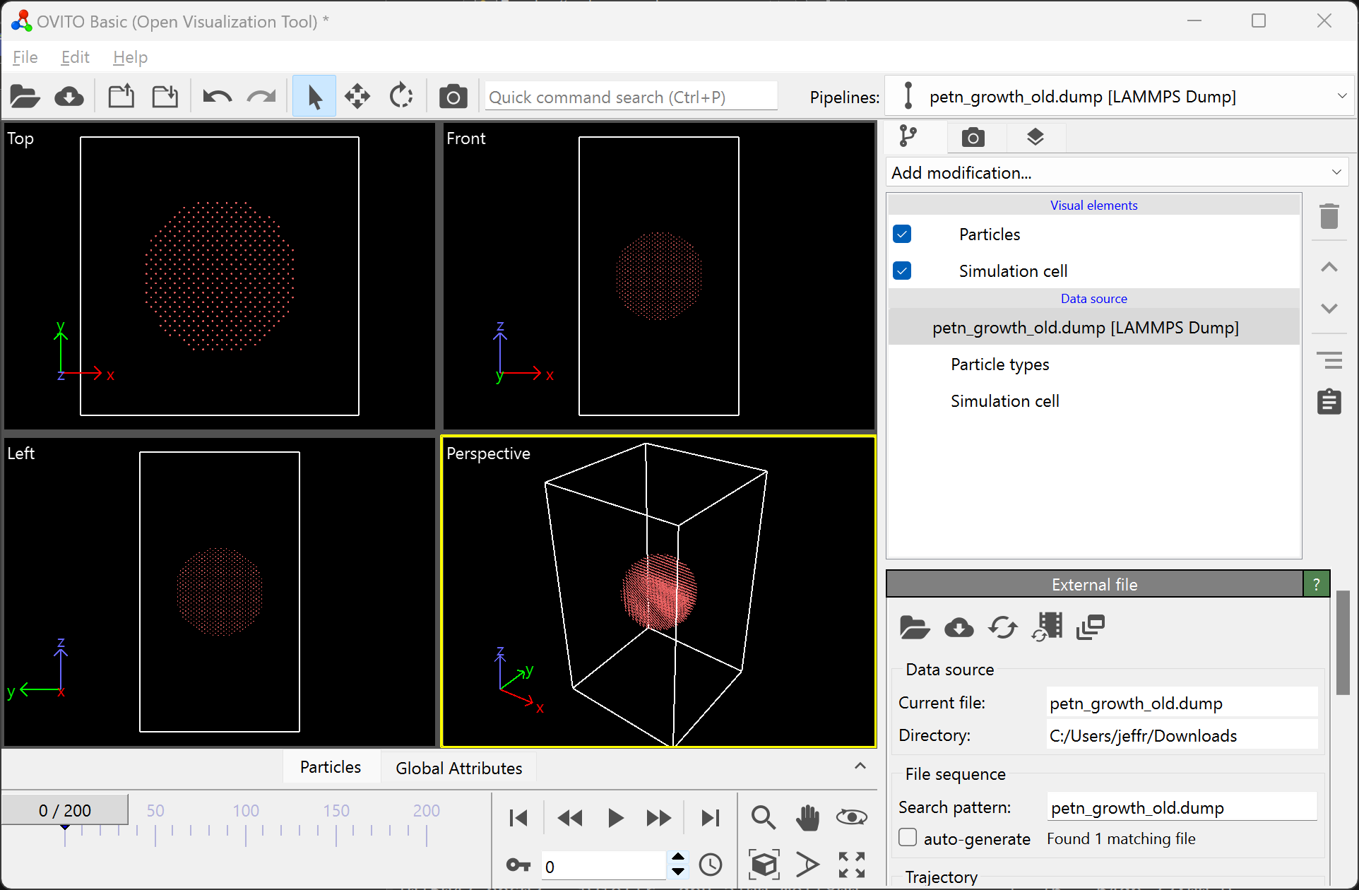
OVITO works particularly well with this tool since it has an internal tool for creating a surface mesh. To visualize your data with a surface mesh, open OVITO and load in the output dump file:
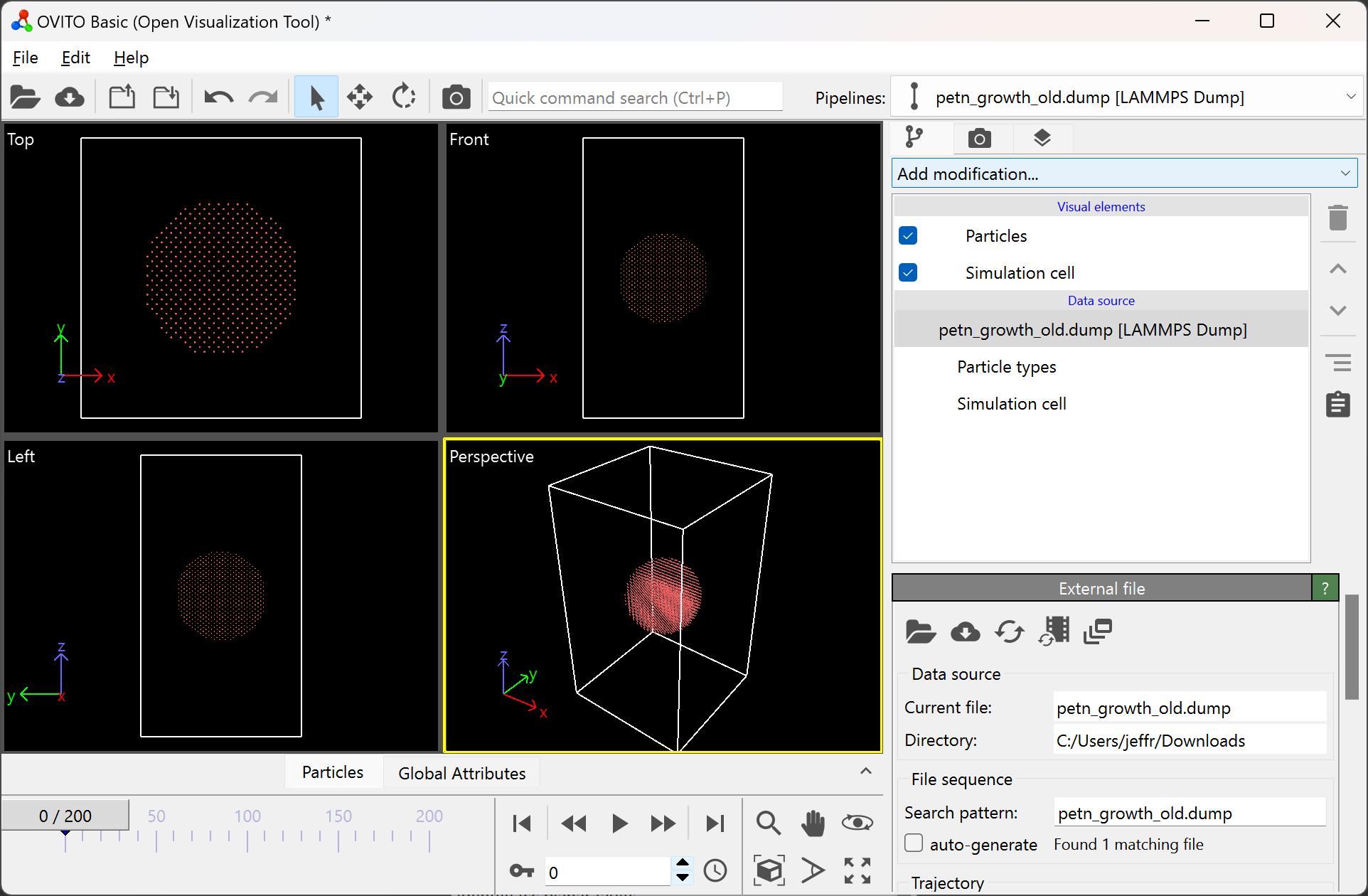
Then, add the “Construct surface mesh” modification:

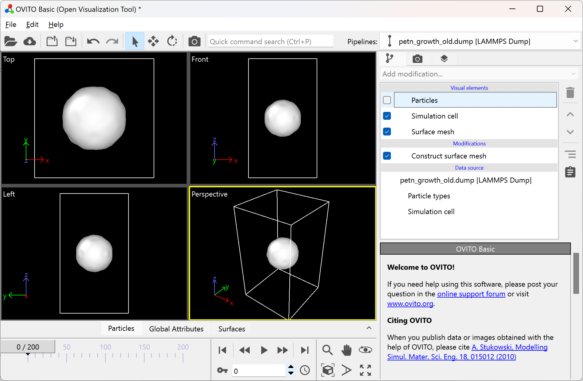
After adding this modification, your OVITO window should look like:

To remove the particles in the visualization window, simply untick the “Particles” option in the top right:
If your surface mesh looks undesirable, try modifying the parameters of the modification. You can do this by clicking on the surface mesh modification, and modifying the available parameters in the bottom right.
In this menu, you can also change the color of the mesh. If your intent is to use these images in a figure, be sure the color contrasts well with a white background.
Once your surface has a desirable shape and color, you can press the play icon to view the time evolution of the surface:

For information on how to render figures and/or movies, visit the OVITO documentation on rendering.
Encapsulating orthogonal vectors
Code for finding encapsulating orthogonal vectors for a given lattice. Enter a given direction (surface normal) to be given two orthogonal vectors. Scalars will be generated that correspond to an error value. The error value is related to the periodicity of the orthogonal vectors.
- Components in directory:
README.md- detailsorth_calc.cxx, func_v.h - source coderun.sh- example run scriptlatticefile.dat- read in lattice vector file from command lattice=read
Compile the code with:
$ g++ -std=c++11 orth_calc.cxx
see run.sh for example on commandline inputs
Inputs:
nx- x value for direction of interest (numerical)
ny- y value for direction of interest (numerical)
nz- z value for direction of interest (numerical)
random- Selects random direction of interest (yes, no)
lattice- lattice vector input (fcc, bcc, cubic, read)
t- lattice vector scalar (numerical)
tmax- Max scalar length for direction of interest (numerical > 0)
tstart- Starting scalar for direction of interest (numerical > 0)
tol- Tolerance for Error function (numerical)
tstep- Loops through tsart to tmax with this step (numberical > 0)